
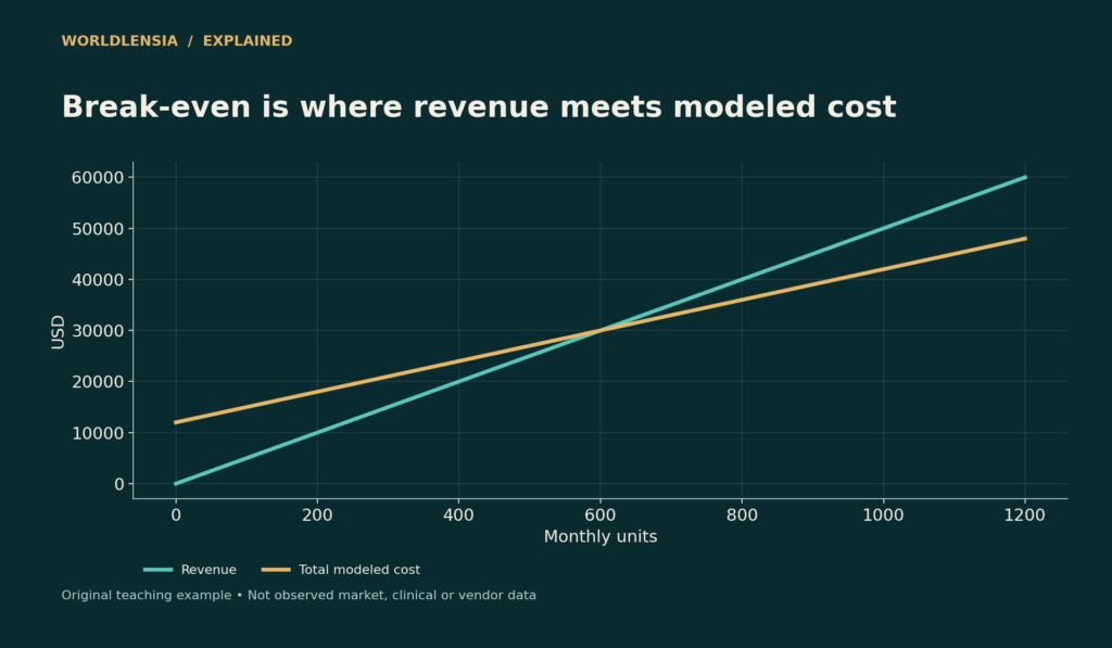
A break-even calculation answers a narrow but useful question: how much must a business sell for revenue to cover the costs included in the model? It does not establish that customers will buy that quantity, that the business has enough cash, or that the owner will receive a suitable return.
The basic calculation divides fixed costs by contribution per unit. Contribution per unit is selling price minus variable cost per unit. A useful analysis then tests the assumptions: selling prices can change, costs can step upward, products have different margins, and available capacity can constrain sales.
This guide develops an original fictional business example. All prices, volumes, costs, and operating assumptions are illustrative. They are not industry benchmarks, a forecast for a particular company, or personalized financial advice.
Build the base case
Imagine a seller with monthly fixed costs of $12,000. Each product sells for $50 and has $30 in variable costs. Each sale contributes $20 toward fixed costs and then profit. Break-even volume is $12,000 ÷ $20 = 600 units per month.
At 600 units, revenue is $30,000, variable costs are $18,000, and total modeled costs are $30,000. At 800 units, revenue is $40,000, variable costs are $24,000, and modeled profit is $4,000 after fixed costs.
| Monthly units | Revenue | Variable costs | Fixed costs | Modeled profit |
|---|---|---|---|---|
| 400 | $20,000 | $12,000 | $12,000 | −$4,000 |
| 600 | $30,000 | $18,000 | $12,000 | $0 |
| 800 | $40,000 | $24,000 | $12,000 | $4,000 |
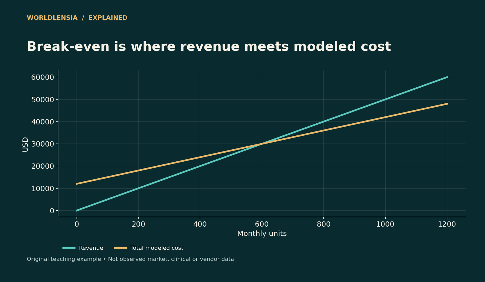
Figure data and assumptions
Original hypothetical teaching data; see the caption and article for assumptions.
| Monthly units | Revenue | Total modeled cost |
|---|---|---|
| 0.0 | 0.0 | 12000.0 |
| 20.0 | 1000.0 | 12600.0 |
| 40.0 | 2000.0 | 13200.0 |
| 60.0 | 3000.0 | 13800.0 |
| 80.0 | 4000.0 | 14400.0 |
| 100.0 | 5000.0 | 15000.0 |
| 120.0 | 6000.0 | 15600.0 |
| 140.0 | 7000.0 | 16200.0 |
| 160.0 | 8000.0 | 16800.0 |
| 180.0 | 9000.0 | 17400.0 |
| 200.0 | 10000.0 | 18000.0 |
| 220.0 | 11000.0 | 18600.0 |
| 240.0 | 12000.0 | 19200.0 |
| 260.0 | 13000.0 | 19800.0 |
| 280.0 | 14000.0 | 20400.0 |
| 300.0 | 15000.0 | 21000.0 |
| 320.0 | 16000.0 | 21600.0 |
| 340.0 | 17000.0 | 22200.0 |
| 360.0 | 18000.0 | 22800.0 |
| 380.0 | 19000.0 | 23400.0 |
| 400.0 | 20000.0 | 24000.0 |
| 420.0 | 21000.0 | 24600.0 |
| 440.0 | 22000.0 | 25200.0 |
| 460.0 | 23000.0 | 25800.0 |
| 480.0 | 24000.0 | 26400.0 |
| 500.0 | 25000.0 | 27000.0 |
| 520.0 | 26000.0 | 27600.0 |
| 540.0 | 27000.0 | 28200.0 |
| 560.0 | 28000.0 | 28800.0 |
| 580.0 | 29000.0 | 29400.0 |
| 600.0 | 30000.0 | 30000.0 |
| 620.0 | 31000.0 | 30600.0 |
| 640.0 | 32000.0 | 31200.0 |
| 660.0 | 33000.0 | 31800.0 |
| 680.0 | 34000.0 | 32400.0 |
| 700.0 | 35000.0 | 33000.0 |
| 720.0 | 36000.0 | 33600.0 |
| 740.0 | 37000.0 | 34200.0 |
| 760.0 | 38000.0 | 34800.0 |
| 780.0 | 39000.0 | 35400.0 |
| 800.0 | 40000.0 | 36000.0 |
| 820.0 | 41000.0 | 36600.0 |
| 840.0 | 42000.0 | 37200.0 |
| 860.0 | 43000.0 | 37800.0 |
| 880.0 | 44000.0 | 38400.0 |
| 900.0 | 45000.0 | 39000.0 |
| 920.0 | 46000.0 | 39600.0 |
| 940.0 | 47000.0 | 40200.0 |
| 960.0 | 48000.0 | 40800.0 |
| 980.0 | 49000.0 | 41400.0 |
| 1000.0 | 50000.0 | 42000.0 |
| 1020.0 | 51000.0 | 42600.0 |
| 1040.0 | 52000.0 | 43200.0 |
| 1060.0 | 53000.0 | 43800.0 |
| 1080.0 | 54000.0 | 44400.0 |
| 1100.0 | 55000.0 | 45000.0 |
| 1120.0 | 56000.0 | 45600.0 |
| 1140.0 | 57000.0 | 46200.0 |
| 1160.0 | 58000.0 | 46800.0 |
| 1180.0 | 59000.0 | 47400.0 |
| 1200.0 | 60000.0 | 48000.0 |
The chart shows where revenue and total cost intersect under these assumptions. It is a model, not evidence that 600 units can actually be sold. Demand must be investigated separately.
Classify costs for the chosen period
Fixed means fixed with respect to the activity and time horizon being modeled. A monthly lease can be fixed over a range of sales, while a packaging charge varies with units. Some costs contain both elements, such as a service with a base fee plus a transaction charge.
Classify costs consistently rather than treating every familiar accounting expense as automatically fixed or variable. Include shipping subsidies, payment processing, packaging, expected returns, sales commissions, and other relevant costs when they change with sales. Avoid counting the same expense in both categories.
The time unit must also match. Annual insurance included in monthly fixed costs needs an appropriate monthly allocation. A quarterly expense cannot be inserted unchanged into a monthly calculation. A timing allocation for profit analysis is not necessarily the same as the cash payment schedule.
Contribution margin is not gross margin
Gross profit depends on the business's accounting classification of cost of goods sold. Contribution analysis focuses on which costs vary with the activity. The two can differ. A product with an attractive gross margin may contribute less after variable selling and fulfillment costs.
For example, if the $30 variable cost excludes a $3 shipping subsidy and a $2 transaction-related cost, actual contribution under the expanded model is $15 rather than $20. Break-even volume becomes 800 units. The difference comes from an incomplete cost model, not a change in the formula.
WorldLensia's margin-versus-markup guide covers a related pricing distinction. Neither a markup percentage nor a gross-margin percentage can be substituted for unit contribution without examining the included costs.
Price discounts require a volume test
Suppose price falls from $50 to $45 while variable cost stays $30. Contribution falls from $20 to $15, a 25% decline. Break-even rises from 600 to 800 units, a 33.3% increase. A 10% price discount therefore requires a much larger proportional increase in break-even volume in this example.
If the seller originally expected 800 units and $4,000 of profit, maintaining that profit at the discounted price requires ($12,000 + $4,000) ÷ $15, or 1,066.7 units. Because whole products are sold, at least 1,067 units are needed under the simple model.
The discount might still be worthwhile if supported by demand, capacity, and cash evidence. The calculation simply makes the required volume visible. Do not assume that every price reduction creates enough additional demand to compensate for reduced contribution.
A cost increase can have the same effect
If price stays $50 but variable cost rises from $30 to $35, contribution again becomes $15 and break-even becomes 800 units. A relatively small change in the cost line can matter substantially when contribution is narrow.
Test cost changes individually and together. A shipping increase, a rise in return rates, and a promotional discount may occur simultaneously. A model that changes only one assumption can understate the combined pressure.
Do not call a sensitivity result a forecast. It says what follows if the assumptions occur. A forecast needs a defensible view of how likely the assumptions are and how they may interact.
Calculate a target profit transparently
To include a desired modeled profit, add it to fixed costs before dividing by contribution. At a $20 contribution and $12,000 fixed costs, a $6,000 target requires 900 units. That is a sales requirement under the model, not a promise of owner take-home pay.
State whether the profit target is before or after taxes, owner compensation, financing costs, and other items. If those are omitted, say so. A small business owner can otherwise mistake an operating result for cash they can safely withdraw.
If contribution is zero or negative, the usual positive break-even volume does not exist under the assumed cost structure. Selling more would not cover fixed costs through positive contribution. Investigate price, variable costs, product design, or the purpose of the transaction before displaying a meaningless result.
The sales mix changes the answer
A business selling multiple products cannot always use one product's contribution for the whole company. Suppose Product A contributes $20 per unit and Product B contributes $10. At a 50:50 unit mix, average contribution is $15. Covering $12,000 requires 800 units in total under that assumed mix.
If the mix shifts to 25% A and 75% B, average contribution becomes $12.50 and the requirement becomes 960 units. Total sales can rise while profit disappoints if the extra volume comes mainly from lower-contribution items.
Keep unit mix separate from revenue mix. Products with different prices can have very different shares of units and revenue. A weighted calculation should state what is being weighted and why that matches the business model.
Capacity can make the target impossible
Suppose the business can fulfill only 700 units per month. The base-case break-even of 600 is physically possible within that capacity. The discounted-price break-even of 800 is not, unless the business changes its process or capacity.
Expanding capacity may add a fixed cost. If an extra shift or facility raises fixed costs, calculate a new break-even for that operating range. Do not use the old fixed cost while assuming access to the new capacity for free.
The bottleneck can be labor, equipment, storage, customer demand, or a supplier. A chart of required sales is useful only when compared with the actual constraint. WorldLensia's capacity-utilization guide discusses why aggregate capacity and the limiting stage can differ.
Step costs break the single straight line
The simplest graph draws fixed costs as unchanged and variable costs as proportional. Real operations can have thresholds. Hiring an additional supervisor after a certain volume creates a step, while bulk purchasing can change unit costs.
Model separate ranges with their own assumptions. If fixed costs rise at 750 units, calculate profit immediately below and above the threshold. A quantity that appeared profitable under the first range may look different once the new cost is included.
Avoid extrapolating the line far beyond the range supported by evidence. A useful model is explicit about where its assumptions apply. More decimals do not compensate for using the wrong operating range.
Break-even is not cash-flow break-even
A company can cover modeled operating costs and still run short of cash. Inventory may be paid for before sale, customers may pay later, and equipment purchases can create large cash outflows. Profit allocation and cash timing differ.
Build a cash schedule alongside the contribution model. Record inventory payments, customer collections, supplier terms, loan payments, and major purchases. WorldLensia's cash-conversion-cycle guide explains why growth itself can tie up cash.
Conversely, an upfront customer payment can improve short-term cash while leaving a future delivery obligation. A positive bank balance does not establish that the business has earned a profit or can distribute the money without considering commitments.
Put returns and defects into the model

Figure data and assumptions
Original hypothetical teaching data; see the caption and article for assumptions.
| Category | Break-even units | Units for $4,000 profit |
|---|---|---|
| $50 price | 600.0 | 800.0 |
| $45 price | 800.0 | 1066.6666666666667 |
If some sales are refunded, gross orders are not identical to completed economic sales. Estimate the revenue retained and costs incurred using a consistent definition. Some returned inventory may be resold; other units may be damaged or incur additional handling.
Avoid subtracting the full sales value and then subtracting the same lost revenue again through another adjustment. A simple transaction-level worksheet can help identify which costs are incurred on every order and which occur only on returns.
For uncertainty, test a plausible range of return rates rather than one precise-looking value. Use actual records where available and disclose when assumptions are based on limited experience. Do not invent an industry average to fill a gap.
Separate acquisition costs from repeat sales
A promotion can produce an initial sale with little contribution while a customer later buys again. That possibility should be evaluated with customer evidence, not assumed. Break-even based on a future customer lifetime value requires its own retention and margin assumptions.
Distinguish an acquisition expense charged once from a cost that recurs on every transaction. Test how quickly contribution is collected and whether customers actually return. If the business cannot fund the period before repeat purchases, an attractive long-term model may still be impractical.
WorldLensia's cohort-retention guide explains why new customers must not be mixed into the denominator when measuring the behavior of an existing group. That distinction helps keep future-revenue assumptions grounded.
A sensitivity table is more useful than a magic number
Create rows for alternative selling prices and columns for variable costs. Calculate contribution and break-even for each combination, flagging impossible or negative-contribution cases. Then compare the required volumes with demand and capacity.
For a board or operating report, highlight the assumptions that drive the largest changes. A small fixed-cost adjustment may matter less than a modest price or variable-cost change. The table should direct investigation rather than create a false impression that every scenario is equally likely.
Keep a base case, a downside case, and clearly explained alternatives. Avoid naming one scenario “conservative” without showing why its inputs deserve that label. An apparently cautious sales estimate can still rely on optimistic costs.
Evidence to collect before acting
Gather actual transaction prices after discounts, cost records, delivery charges, return outcomes, staffing limits, supplier lead times, and payment timing. Reconcile totals against accounting records while preserving the contribution classifications used in the model.
Then test the model against a completed period. Compare predicted and actual revenue, variable costs, and profit. Investigate differences before using it for a larger commitment. A useful model improves through reconciliation rather than through presenting an increasingly elaborate forecast.
Questions to ask before approving a plan
Are fixed costs and sales in the same time period? Does the contribution include every relevant variable cost? Is the sales mix realistic? Can capacity handle the required volume? Does cash arrive early enough to fund operations? What happens if price falls or costs rise?
Also ask what evidence would cause the plan to change. A model should help decide whether to revise pricing, reduce costs, limit a promotion, or postpone expansion. If every scenario leads to the same predetermined decision, the spreadsheet is serving as decoration.
Calculate the margin of safety
If expected sales are 800 units and modeled break-even is 600, the unit margin of safety is 200. As a share of expected sales it is 200 ÷ 800 = 25%. Under unchanged price and cost assumptions, sales could fall by that proportion before the modeled result reaches zero.
This is not a probability that the business will remain profitable. It does not estimate how likely the sales decline is, and it does not account automatically for changes in costs or mix. Label it as a distance from a modeled threshold.
In the discounted-price scenario, break-even rises to 800. At the same expected 800 units, the modeled margin of safety disappears. The comparison makes the operating consequence of the discount visible without claiming that demand will or will not respond.
Analyze a service business in hours
The contribution logic can apply to a fictional service with $8,000 of monthly fixed costs, a $100 billable hourly price, and $40 of variable cost per billable hour. Contribution is $60 per billable hour, so the simple break-even requirement is 133.33 hours, or at least 134 if only whole hours are sold.
But billable hours are not identical to all working hours. Administration, sales, training, and rework can reduce the portion available for clients. If only 120 billable hours are realistically available, the target is infeasible under that capacity and pricing structure.
This example does not prescribe an hourly rate. It shows how a unit should match the business activity. A project-based service may need project contribution or a mix of hours and fixed deliverables rather than a retail product formula copied unchanged.
Investigate a zero-profit result before calling it sustainable
Covering the costs included in a model may leave out the owner's labor, replacement of equipment, or a return for risk. A zero at the bottom of an incomplete model is not evidence that the business supports its owner or can renew its assets.
Write down the scope. An operating contribution model can be useful even when it omits financing and taxes, provided the result is labeled correctly and those other obligations are assessed elsewhere. Confusion arises when a narrow break-even is presented as complete financial sustainability.
Also distinguish accounting depreciation from cash needed for replacement. The appropriate treatment depends on the question being asked. A long-term plan should not assume that equipment lasts forever because a short-run contribution calculation does not include a new purchase.
Review incentives created by the target
A sales quota based on gross units can encourage discounting that reduces contribution. A production quota can encourage inventory accumulation even when customers have not bought the goods. The performance measure should reflect the actual economic objective.
For example, selling 1,000 units at a $10 contribution generates the same total contribution as 500 at $20, before any differences in fixed costs or constraints. The larger unit count is not automatically the stronger outcome. Cash timing, capacity use, returns, and customer effects can distinguish them further.
Use the model to ask which sales are valuable under the actual constraints. A bottleneck hour spent on a low-contribution product may crowd out a more valuable use. That requires product-level and process evidence rather than a blanket instruction to maximize volume.
Keep a change log for the model
Record when price assumptions, cost classifications, sales mix, and capacity were updated. Preserve the earlier version used for an actual decision so later results can be compared with what was known at the time.
When actual results differ, separate input errors from calculation errors and genuine business changes. A formula can be correct while the demand assumption is wrong. The remedy is then better evidence or a revised plan, not merely a more elaborate spreadsheet.
Distinguish a planning buffer from a verified expense
A model can include an explicit contingency allowance for uncertain costs. Keep that allowance visible rather than hiding it inside an unrelated line. Otherwise later reviewers cannot tell whether an increase reflects a known contract price or a precautionary assumption.
Test the allowance separately and reconcile it after actual results arrive. A buffer can improve planning discipline, but it does not guarantee that every adverse event fits within it. The relevant question remains whether the business can fund a plausible downside case while meeting its other obligations.
Do not present the resulting break-even as exact to a fraction of a product when several inputs are rough estimates. Round operational requirements appropriately and explain the uncertainty in the assumptions that drive them.
Practical conclusion
Use break-even analysis to expose the relationship among contribution, fixed costs, volume, and capacity. Keep the formula simple and the assumptions visible. Pair it with demand evidence and a cash schedule before treating the required sales level as achievable.
The result is most useful as a range of clearly explained conditions. It tells the reader what must be true, what could change the answer, and which operational records need to be checked next.
Check the rounding boundary
If the formula produces 600.2 units and products are indivisible, 600 units do not quite cover the modeled costs. Round the required quantity upward under that assumption. For a service sold in fractional hours, the relevant billing increment can differ. State the operational rule rather than rounding automatically to the nearest whole number. Also distinguish a mathematical minimum from a practical target with a planning buffer. The buffer reflects uncertainty or operational preference; it should not be hidden inside the formula and described as if it were a measured expense.
Sources and methodology
SBA break-even resources and OpenStax managerial-accounting explanations were checked October 18, 2026. All numerical examples, scenario comparisons, and operating constraints here are original calculations using fictional inputs. No sales forecast or industry benchmark is asserted.
- SBA: Business planning and break-even — checked October 18, 2026.
- OpenStax: Break-even in units and dollars — checked October 18, 2026.
Continue with Gross margin versus markup and Cash conversion cycle for related context.
To connect break-even assumptions with pricing and incremental cost, see Gross Margin vs Markup: Price a Product Without Mixing Formulas and Allocated Cost and Incremental Cost Answer Different Decisions.