
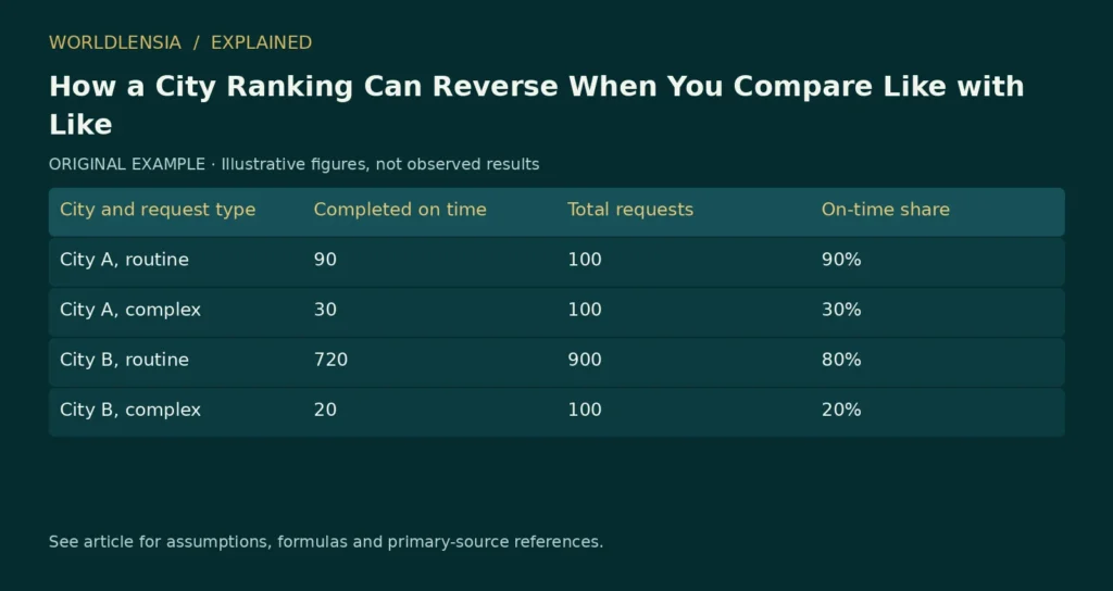
An overall city ranking can reverse within every relevant subgroup because the cities serve different mixes of cases. This arithmetic pattern is commonly called Simpson’s paradox. It warns that an aggregate percentage may answer a different question from a comparison within comparable groups.
The appropriate response is not to assume that the subgroup result is always correct. First define the question and understand how the data were generated. A population’s actual experience and a comparison under a common case mix can both be useful, but they are different quantities.
A city ranking example with two service groups
Imagine two cities processing routine and complex service requests. We want to compare the share completed on time. All counts below are invented for explanation; they do not describe any real city or agency.
| City and request type | Completed on time | Total requests | On-time share |
|---|---|---|---|
| City A, routine | 90 | 100 | 90% |
| City A, complex | 30 | 100 | 30% |
| City B, routine | 720 | 900 | 80% |
| City B, complex | 20 | 100 | 20% |
City A has a higher on-time share for both routine and complex requests. Yet its overall share is 120/200 = 60%, while City B’s is 740/1,000 = 74%. The overall ranking favors City B.
The reason is the mix. Half of City A’s requests are complex, compared with one tenth of City B’s. Routine cases have higher on-time shares in both cities. City B’s aggregate benefits from having more of them.
How a city ranking can reverse despite subgroup results
City A’s overall rate is 0.5 × 90% + 0.5 × 30% = 60%. City B’s is 0.9 × 80% + 0.1 × 20% = 74%. Each city’s rates are combined using its own case shares.
If we apply the same illustrative 50/50 weights to both, City A remains at 60% and City B becomes 0.5 × 80% + 0.5 × 20% = 50%. Under that common mix, City A has the higher rate.
Neither calculation erases the actual 74% experienced across City B’s observed requests. The standardized calculation answers a hypothetical comparison: what would the rate be if each city’s subgroup rates were applied to the same specified mixture?
Research on Simpson’s paradox discusses why interpretation depends on the structure of the problem, especially when people try to turn associations into causal conclusions. [1] The arithmetic identifies a possible composition effect; it does not identify the correct policy response by itself.
A separate aggregation problem arises when a place-level association is used to describe individuals. Our county health map guide explains why an area-level pattern does not identify individual risk.
Decide which question you are asking
If a resident asks what proportion of all requests were completed on time in each city, the observed aggregate is directly relevant. If an analyst asks how the cities compare for similar types of requests, subgroup results or an appropriately standardized measure may be more useful.
If the question is whether a management reform caused better performance, neither table alone settles it. Differences in staffing, reporting rules, resources, case difficulty within each label and other factors could matter.
The word “complex” also needs a reproducible definition. If one city classifies difficult cases as routine and another uses a broader complex category, the subgroup comparison can remain misleading. Better labels do not automatically create comparable groups.
Do not average percentages without their counts
An unweighted average of City B’s two subgroup rates is 50%. That happens to match the common 50/50 calculation above, but it does not equal City B’s observed overall rate of 74%.
To calculate the actual combined rate, sum the numerators and denominators: (720 + 20)/(900 + 100). Averaging 80% and 20% implicitly gives equal weight to categories containing very different numbers of requests.
This problem appears in many local comparisons: service completion, housing applications, school attendance, business formation and transport use. The specific interpretation changes, but the need to preserve counts and population definitions remains.
Check whether the groups are appropriate
Subgroup analysis should follow a reasoned measurement plan. Repeatedly dividing a dataset until a preferred ranking appears is not a reliable method. Categories should relate to the substantive question and have enough evidence to support interpretation.
Small groups can also be noisy. If a city has only a few complex requests, its estimated rate may vary sharply. Show counts and uncertainty when appropriate, and distinguish observed administrative totals from survey estimates.
For survey-based city comparisons, the Census Bureau’s ACS comparison guidance provides checks on estimate type, period and reliability. [2] A mathematically correct weighted average cannot repair incompatible survey universes or geographic boundaries.
How to audit a city ranking comparison
Present the overall rate alongside the main subgroup rates and case shares. If you publish a standardized comparison, name the reference weights and explain why they suit the question. Do not label an adjusted rate as though it were the directly observed experience of residents.
A short note can say: “The observed total uses each city’s own request mix. The common-mix illustration applies equal weights to routine and complex cases.” That sentence tells readers why the two rankings differ.
Our guide to population density and weighting explores a related issue: the choice of weights changes the quantity being summarized. Here, case shares determine the overall rate; elsewhere, people, households or land area may be the appropriate weights.
The practical lesson is to investigate a ranking’s denominator and composition before explaining it. A reversal does not mean arithmetic failed. It means the aggregate and subgroup comparisons combine information differently, and the reader needs the underlying structure to decide which comparison answers the intended question.
Reconstruct the comparison from the original counts
A reproducible worksheet should begin with counts rather than typed percentages. Enter on-time completions and total requests separately for every city and request type. Calculate each rate from those inputs, then calculate the aggregate from summed counts.
For City A, the numerator is 90 + 30 = 120 and the denominator is 100 + 100 = 200. For City B, the numerator is 720 + 20 = 740 and the denominator is 900 + 100 = 1,000. These totals reproduce 60% and 74%.
Next, calculate the subgroup shares. City A’s routine share is 100/200 = 50%. City B’s is 900/1,000 = 90%. These are the weights used by the observed aggregate, not arbitrary analyst choices.
Keeping these steps separate helps identify a common spreadsheet mistake: averaging subgroup rates to recreate an observed total. That only works when the subgroup denominators happen to imply equal weights or when the analyst explicitly wants an equal-weight hypothetical.
Test several common reference mixes
The 50/50 illustration is one possible reference. A comparison can also use the pooled mix of all observed requests, provided the choice is appropriate and explained. Here, the pooled routine count is 100 + 900 = 1,000, and the pooled complex count is 100 + 100 = 200.
The pooled weights are therefore five sixths routine and one sixth complex. Applying them to City A gives (5/6 × 90%) + (1/6 × 30%) = 80%. Applying them to City B gives (5/6 × 80%) + (1/6 × 20%) = 70%.
The common-mix ranking again favors City A, but the levels differ from the 50/50 illustration. A standardized rate needs its reference weights to be interpretable. “Adjusted performance” without the adjustment definition is not a sufficient label.
In this particular synthetic example, City A’s rate exceeds City B’s by ten percentage points in both subgroups. Consequently, any common mixture of these two subgroup rates preserves that ten-point gap. That property follows from the invented numbers; it is not a general guarantee for real comparisons where subgroup gaps differ.
Separate the resident-experience question from the service-comparison question
A resident asking about the observed probability of an on-time completion among all recorded requests may reasonably care about the aggregate. A manager comparing performance on similar workloads may care about the subgroup or standardized result.
The first question uses the actual mixture of cases. The second deliberately holds some aspect of the mixture constant. Neither calculation should be used to dismiss the other as fake. Their meanings differ.
A practical article can show both: observed overall results and a clearly labeled common-mix illustration. Then explain that the latter is a descriptive standardization, not an estimate of what would certainly happen if the cities exchanged workloads.
Changing a city’s case mix could also change staffing needs, queues and outcomes. Applying existing subgroup rates to a new mix holds those rates fixed by assumption. That is useful for a teaching calculation but may be unrealistic as a policy forecast.
A classification rule can create another comparability problem
Suppose City A calls a request complex whenever it needs an external approval, while City B uses the label only when it also requires a site visit. The two complex categories no longer represent the same type of case.
A within-category comparison can then remain confounded by differences hidden inside the labels. Standardization using incompatible categories gives a precisely calculated result for a poorly defined comparison.
Before using the table, write a common classification rule and determine whether both sources support it. If the original records cannot be reclassified consistently, state the limitation. Do not invent a mapping merely to produce a clean ranking.
The same issue can arise with an outcome definition. One city may pause the completion clock while awaiting information; another may include that time. Their on-time rates would describe different rules. Align the measurement before interpreting performance.
Examine missing and excluded requests
A reported service rate can omit open cases, withdrawn requests or records lacking a completion date. Those exclusions affect the population being summarized. A city with more unresolved cases can appear different if only completed cases enter the denominator.
For a fictional illustration, imagine 100 additional City B requests still open and excluded from the original table. The existing 74% describes the stated 1,000-record population. It does not automatically describe all 1,100 requests received.
Do not simply count all open requests as failures unless that matches the defined outcome and deadline. Instead, identify which requests have had enough time to be evaluated and preserve unresolved status. A cohort based on receipt date can be useful when the question concerns all incoming work.
A source note should state inclusion, exclusion and outcome-maturity rules. Without them, the apparent composition effect may be mixed with a reporting-population difference.
Avoid selecting subgroups after seeing the desired result
An analyst can divide data in many ways: request type, district, channel, month or staff team. Searching these splits until a preferred city leads creates a risk of selective explanation.
Choose substantively relevant categories before interpreting the result where possible. If an exploratory split reveals a pattern, label it exploratory and test it with additional appropriate evidence. Do not present it as an independently confirmed explanation merely because the arithmetic is correct.
A useful review asks whether the categories reflect factors present before the outcome and whether they fit the substantive question. Some variables can be affected by the process being evaluated, so controlling for them can change the question rather than simply improve fairness.
This is one reason causal interpretation needs more than a disaggregated table. The decision about what to compare must reflect how the system works.
Show sensitivity without creating a forest of charts
For mobile readers, three compact rows may be enough: observed aggregate, equal-mix illustration and pooled-mix illustration. Include the reference weights and keep percentages on a common scale.
The corresponding synthetic rates are A 60% versus B 74% for observed totals; A 60% versus B 50% for equal weights; and A 80% versus B 70% for pooled weights. The first row uses different weights for each city; the other rows use common weights.
That difference should be explicit in the table header or caption. Otherwise a reader may think the same population has three contradictory rates. They are three different summaries built from the same subgroup inputs.
Include the original count table nearby. An explanatory chart is easier to trust when readers can reconstruct it. Color can distinguish cities, but labels should carry the meaning without relying on color alone.
Identify what an uncertainty analysis would require
The synthetic example uses fixed invented counts to demonstrate arithmetic. It does not include a sampling design. A real analysis needs to identify whether the counts are administrative totals, survey estimates or sampled audit results.
If they are survey estimates, use the appropriate design-aware uncertainty method. If they are administrative counts, measurement and coverage errors can still matter even when conventional sampling uncertainty is not the main issue.
Do not attach an arbitrary confidence interval to the fictional rates and present it as an official method. Likewise, a statistically distinguishable rate difference does not by itself establish a causal management effect.
Uncertainty should be connected to the quantity being estimated. A standardization that estimates a hypothetical common-mix rate can require additional assumptions and covariance information. A transparent article can explain the arithmetic while leaving formal inference to a method supported by the actual dataset.
Turn the comparison into an editorial checklist
Before publication, ask whether the headline names the measured population, whether all subgroup counts reconcile and whether the weight choice is visible. Check that a common-mix result is labeled hypothetical or standardized rather than observed.
Then ask whether the article makes an unsupported causal leap. “The aggregate differs because the illustrated mix differs” is an arithmetic explanation within the example. “Changing management would produce a ten-point improvement” would require evidence beyond this table.
Finally, inspect the labels for value judgments. A higher completion share under one measure does not summarize all dimensions of service quality. Speed, accuracy, accessibility, cost and resident satisfaction can differ. Do not call a city universally better from one rate.
Preserve a useful result when the ranking remains uncertain
An investigation can be valuable even if it cannot produce a definitive winner. It may establish that the raw totals reflect different case mixes, that outcome rules need alignment or that one segment lacks enough evidence.
Those findings tell readers what the numbers mean and what additional information would improve the comparison. They can also guide a data request without inventing missing values.
The strongest explanation follows the full chain: define the question, identify the population, calculate the subgroup rates, show the weights and state the interpretation. A ranking reversal then becomes understandable. It is evidence that aggregation choices matter, not permission to choose whichever summary supports a preferred story.
A reader exercise with a different reference population
Use a reference mix containing 25% routine and 75% complex requests. Applying the original fictional subgroup rates gives City A 0.25 × 90% + 0.75 × 30% = 45%. City B gives 0.25 × 80% + 0.75 × 20% = 35%.
The standardized levels are lower than under the pooled reference because the new reference gives more weight to complex requests, which have lower on-time shares in both cities. The ten-point gap remains because of the way the example’s subgroup differences were constructed.
Now ask which reference is appropriate for a real decision. Equal weights are easy to explain, pooled weights describe the combined observed case mix, and a planning reference might describe an expected future workload. None should be selected merely because its level looks favorable.
If a proposed future mix is used, label it a scenario and identify its source or assumption. Applying current subgroup rates to it does not establish that the rates would remain fixed after staffing and demand changed.
This exercise also explains why standardized rates from two reports may differ when they use different reference populations. Before declaring a contradiction, compare the reference weights and subgroup definitions.
Keep the original evidence available after publication
Publish or retain a compact machine-readable table of the synthetic inputs, calculation formulas and reference weights. Another reader should be able to reproduce the numbers without interpreting a screenshot of a chart.
For real administrative data, publication may require privacy or licensing controls. A public explanation can still describe the method and source while preserving appropriate restrictions on individual records. Do not imply that transparency requires exposing sensitive case details.
For this educational example, every count is invented and can be shared with its illustrative label. That label belongs in the table, image caption and alt text, so the explanation remains clear when the visual is viewed outside the article.
A final check should confirm that every displayed percentage can be reproduced from its stated counts and weights. If it cannot, correct the table before interpreting the ranking or proposing an explanation.
Sources and method
- Simpson’s paradox in psychological science: a practical guide. August 12, 2013. Checked October 20, 2026.
- Census comparing ACS data. Living guidance; publication date not established. Checked October 20, 2026.
Numerical teaching examples are original and illustrative unless explicitly identified otherwise. No hands-on product testing or individual medical assessment is claimed.
When comparing local growth stories, definitions and population composition matter. For a current example, see our analysis of fastest-growing U.S. cities.
To connect a ranking reversal with uncertainty and distribution, see ACS Margins of Error: When a City Ranking Is Too Precise and Mean vs Median Income: The Average Can Rise While Most Households Stand Still.
Work through the counts: Download the printable city-data activities (PDF, 49 KB). Page 1 includes the fictional request counts, a common-mix exercise and an answer key so you can reconstruct the ranking reversal.