
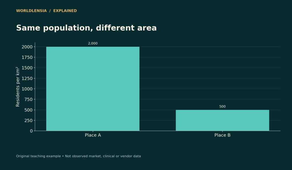
Population density divides a population by an area, but the result depends on both the boundary and the kind of area used. A compact city and a large administrative region can have different average densities even when their residents live in similarly crowded neighborhoods.
The Census Bureau describes population density as the number of people within a defined area, commonly expressed per square mile or square kilometer. That basic ratio is useful. The mistake is assuming it captures every feature of settlement, housing conditions, or service demand.
Population density starts with a transparent ratio
Two fictional places each contain 100,000 residents. Place A covers 50 square kilometers and has a density of 2,000 people per square kilometer. Place B covers 200 square kilometers and averages 500. The population is identical; the denominator creates the fourfold difference.
Now suppose most of Place B's residents occupy 25 square kilometers while the remaining land consists largely of undeveloped areas. Its administrative average does not describe the density of those neighborhoods. Do not divide by an assumed occupied area unless you have defined and measured that area consistently.
| Place | Residents | Administrative land area | Average density |
|---|---|---|---|
| A | 100,000 | 50 km² | 2,000/km² |
| B | 100,000 | 200 km² | 500/km² |
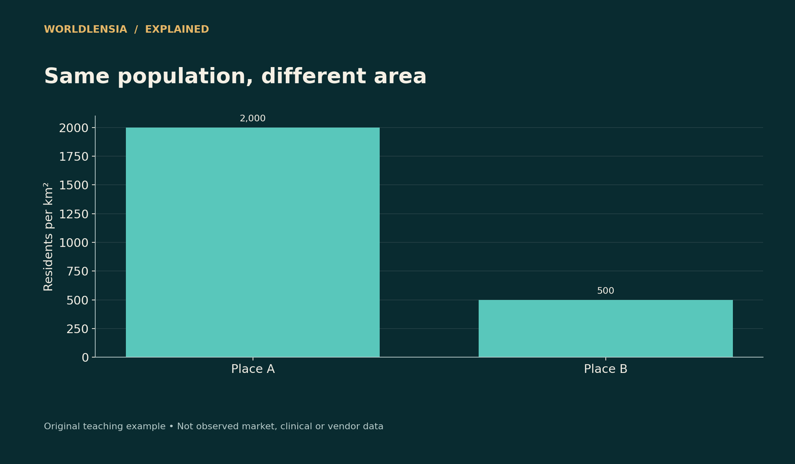
Figure data and assumptions
Original hypothetical teaching data; see the caption and article for assumptions.
| Category | Density |
|---|---|
| Place A | 2000.0 |
| Place B | 500.0 |
The figure illustrates boundary sensitivity, not a real city ranking. Both land-area and population definitions belong beside the result.
Land area and total area differ
If a boundary contains substantial water, using total area produces a different ratio from using land area. Either calculation can be described, but comparing one city's land-based density with another city's total-area density is inconsistent.
Also check the units. One square mile is approximately 2.59 square kilometers. A density expressed per square mile is therefore numerically about 2.59 times the equivalent density per square kilometer. Relabeling the axis without conversion creates a large error.
An average is not the experience of the average resident
Consider two equally sized neighborhoods, one with 9,000 people per square kilometer and another with 1,000. Their area-weighted average is 5,000. But nine out of ten residents live in the denser neighborhood. A population-weighted neighborhood measure would answer a different question about the density surrounding residents.
Neither measure is automatically correct for every purpose. Infrastructure planners may need total service territory; a study of neighborhood exposure may need a population-weighted measure. State the weighting rule so readers can reproduce it.
Density is not the same as household crowding
A high-rise neighborhood can have many residents per square kilometer while providing spacious homes. A lower-density area can contain overcrowded dwellings. Persons per room, household size, unit size, and housing quality address different dimensions.
Avoid inferring unhealthy or inadequate housing from geographic density alone. The relevant evidence might concern ventilation, occupancy, affordability, building conditions, or access to services. A citywide map is a starting point for questions, not a diagnosis of every household. Our county health map guide explains the limits of interpreting area-level health patterns.
Boundaries can create an artificial trend
If a city annexes lightly populated land, its average density can fall without anyone moving out of the original neighborhoods. Conversely, redrawing a boundary around the built-up center can raise the reported density without new construction.

Figure data and assumptions
Original hypothetical teaching data; see the caption and article for assumptions.
| Category | Density |
|---|---|
| Area-weighted | 5000.0 |
| Population-weighted | 8200.0 |
For a historical comparison, use a consistent geography or document the boundary change. Match population dates to the area definition. WorldLensia's city-versus-metro guide explains the related problem of comparing different kinds of geographic units.
What a map adds
A neighborhood population density map can show the spatial pattern hidden by the city average, but its interpretation depends on geographic scale. Large zones smooth local differences; small zones can make estimates noisier or expose privacy concerns. Use a suitable scale and include the source, year, and method.
Do not turn a conceptual illustration into a fictional city map. The visuals here are labeled teaching comparisons. A real map would require actual geographic boundaries and compatible population data.
Compare population density averages with explicit weights
For the two equal-area neighborhoods with densities of 9,000 and 1,000, the population shares are 90% and 10%. Weighting the neighborhood densities by those shares gives 0.9 × 9,000 + 0.1 × 1,000 = 8,200 people per square kilometer.
That does not change the city's total population or land area. It answers a different question about the density of the neighborhoods in which residents live. The 5,000 area-weighted density and 8,200 population-weighted density can both be valid when clearly labeled.
The geographic units still matter. If the dense neighborhood contains a small concentrated residential district and substantial open space, a finer subdivision can change the population-weighted result. Do not claim that one weighted number captures an objective experience independent of scale.
Keep the map legend honest
Use intervals and colors that make comparisons readable without implying unwarranted precision. If the map is based on a survey estimate, include the reference period and uncertainty where relevant. A boundary drawn in fine detail does not make the underlying estimate equally precise.
For changes over time, retain a consistent legend or explain why it changes. Otherwise an area can appear darker simply because the color thresholds moved. Show actual numerical values alongside the visual so readers can check whether the apparent change is real.
Do not use density as an automatic explanation
If denser neighborhoods have shorter commutes in a particular dataset, the relationship may also reflect job locations, transport service, income, land use, and other conditions. The density ratio alone does not isolate a causal effect.
Describe the observed association and the additional analysis needed. A ranking of averages is a descriptive tool, while a claim about what a planning change would cause requires a stronger design. Keeping that distinction visible makes a city article more useful without overstating what a map can prove.
Build a fair density comparison
Record population, reference date, boundary type, land or total area, area units, and any weighting method. Then ask whether density actually answers the reader's question. If the topic is commuting, access, or household crowding, bring in those measures directly.
A good comparison uses density as one defined piece of evidence. It does not use the number as a shortcut for prosperity, livability, or the character of residents.
Use a denominator audit
Before finalizing a density table, verify that the area values are in the stated units and refer to the same boundary date as the population. Check at least one calculation manually. If the source gives both land and total area, document which was selected. A simple audit can catch a square-mile conversion error or a mismatched geography that would otherwise survive into a polished map. The resulting figure should carry its definition in the caption so a shared image remains understandable without the entire article beside it.
Sources and methodology
Census population-density and geographic documentation was checked October 18, 2026. All populations, areas, and neighborhood examples in this article are original hypothetical illustrations.
- Census: Population density — checked October 18, 2026.
Continue with City versus metro boundaries and Surface versus air temperature for related context.
To connect density with geographic boundaries and population composition, see City vs Metro Population: Why the Boundary Changes the Answer and How a City Ranking Can Reverse When You Compare Like with Like.
Practise the comparison: Download the printable city-data activities (PDF, 49 KB). Page 2 works through fictional boundary changes and population-weighted zone densities, with an answer key and the definitions kept beside the calculations.