
A provisional death count reflects records received and processed by a specified date. Recent periods can be incomplete because registration, investigation, coding and reporting take time. A low recent count therefore does not automatically establish a real decline in deaths.
The central comparison is not only between weeks of occurrence. It is also between the reporting maturity of those weeks. An older week may have had many more opportunities for records to arrive than a week that just ended.
Keep two dates in every analysis
The occurrence period describes when deaths happened. The extraction or release date describes when the dataset was observed. Both are needed to reproduce a provisional count.
CDC WONDER’s provisional mortality documentation explains that recent data can be incomplete and provides query and coverage details. [1] An older CDC technical-notes page describes the reporting-lag problem but is explicitly archived and should not be used as a source of current counts. [2]
This article uses fictional records to illustrate revision timing. It does not report a current mortality trend, estimate an individual’s health risk or provide medical advice.
Watch one fictional week mature
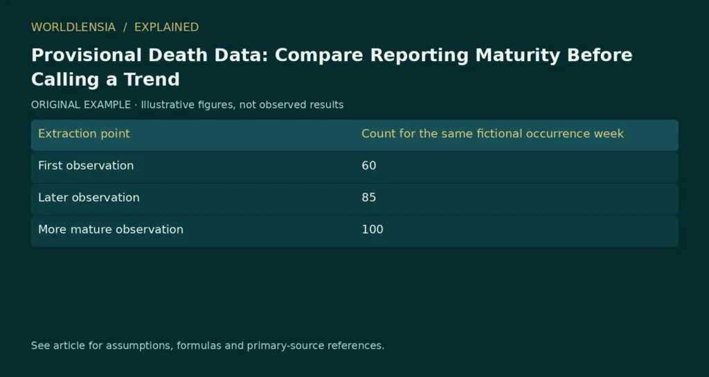
Suppose a week initially appears with 60 recorded deaths. Two weeks later, the same occurrence week has 85, and after additional reporting it has 100.
| Extraction point | Count for the same fictional occurrence week |
|---|---|
| First observation | 60 |
| Later observation | 85 |
| More mature observation | 100 |
The later values do not mean those additional deaths occurred on the extraction dates. They are records assigned to the same earlier occurrence week. A chart should preserve that distinction.
Revisions can also involve corrections, so do not assume every update must increase a count. Read the dataset’s methods and retain the original extract rather than relying on a changing live table alone.
Unequal maturity can create an apparent decline
Imagine comparing a mature earlier week containing 100 records with a just-ended week containing 60. The apparent change is −40%. In the fictional maturation sequence above, the newer week could later reach 100, removing that apparent decline.
That possibility does not prove the actual underlying trend is flat. It shows why incomplete counts cannot be interpreted as complete observations without qualification.
A useful method may compare equal reporting lags, such as each occurrence week as observed the same number of weeks later. Another may use a documented adjustment for completeness. Either approach requires the appropriate data and assumptions; a generic multiplier is not a defensible substitute.
Adjustment adds assumptions, not certainty
A model that estimates incomplete reporting relies on patterns in available data. Changes in reporting processes or cause-specific delays can affect those patterns. If adjusted estimates are used, distinguish them from observed records and show uncertainty where supplied.
Do not take the fictional 60-to-100 relationship here and apply a factor of 1.67 to real recent data. The numbers were invented to explain timing. Real completeness varies by dataset, place, period and other characteristics.
Some causes can require longer investigation. Read the source’s cause-specific release rules and suppression notes before comparing categories. An unavailable cell is not zero, and an intentionally delayed category is not necessarily an observed absence.
Match the rest of the query as well
Use compatible geographic definitions, resident coverage, age groups, cause definitions and occurrence periods. A change in the query can alter counts independently of reporting maturity.
For rates, verify the population denominator and whether the estimate is crude or adjusted. Completeness in the numerator is one issue; comparability of the rate is another. Solving the lag problem does not remove differences in population structure.
Our article on reported and measured health data explains the broader importance of the collection method. Provisional mortality analysis adds a version and timing dimension to that discipline.
Write a source note that can be reproduced
Record the dataset, query filters, occurrence range, extraction timestamp, observed or adjusted status and relevant completeness notes. If later figures differ, the saved extract should make clear whether the difference is a revision or a changed query.
A responsible chart can visually mark recent incomplete periods and explain what evidence is needed before interpreting them. It should not draw a dramatic downward line through the newest weeks without showing the reporting caveat.
The useful conclusion names what is known: how many records were available for a defined period at a defined extraction date. A trend claim needs the additional work of comparing compatible, sufficiently mature observations or using a justified adjustment method.
Build a reporting-maturity matrix
A useful dataset for checking reporting lag stores occurrence periods in rows and extraction dates in columns. Each cell is the count available for the same occurrence period at that extraction date. This keeps revisions visible instead of overwriting them.
For a fictional example, Week A has 60 records after one week, 85 after three weeks and 100 after six weeks. Week B has 66, 90 and 105 at the same lags. Comparing the first-lag counts gives a 10% increase; comparing the six-week counts gives a 5% increase.
The two comparisons use different maturity but each aligns the lag between the weeks. Neither should be described as the final truth unless the source says the observations are final. The exercise shows why both occurrence time and reporting time belong in the data structure.
Distinguish a revision from a new event
If Week A moves from 85 to 100 between extracts, that is a 15-record revision to the same occurrence period. It is not 15 deaths assigned to the later extraction week.
An automated chart that stores only extraction dates can accidentally plot revisions as though they were newly occurring events. Preserve the source’s occurrence variable and use the extraction date as version metadata.
The same principle applies to corrections that reduce a count. A negative revision is not a negative number of deaths occurring today. It is a change in the recorded information for a defined earlier period.
Compare regions with equal care
Suppose two fictional regions have identical underlying events but different reporting speeds. At a short lag, one can appear to have a lower rate merely because fewer records have arrived. A map of the newest period can then partly map reporting processes rather than mortality.
To investigate an actual regional comparison, read the source’s completeness guidance and use a suitable common maturity or documented adjustment. Do not assume a single national completeness pattern applies equally everywhere.
Even after aligning lag, check population coverage, age structure, cause definitions and denominator vintage. A better timing comparison is one necessary step, not a complete comparability guarantee.
Some records may exist before all cause information is complete or available under the release policy. A cause-specific count and an all-cause count can therefore have different timing limitations.
Read whether the source delays publication, suppresses small cells or uses categories for pending information. Preserve these states in the extract. Replacing a delayed value with zero invents information and can produce a false trend.
If a chart excludes a category, disclose the exclusion and avoid describing the remaining sum as a complete total unless the source supports that interpretation.
Write a responsible update note
A recurring article should identify the new extraction date, the occurrence periods added and material revisions to earlier periods. If a previously described decline disappears after maturation, explain the revision and the earlier limitation.
Do not simply change the chart and leave the original causal interpretation intact. The interpretation should follow the current evidence, while the version record preserves what was previously available.
An appropriate correction can be concise: the newest periods were incomplete, later records changed the comparison, and the updated chart now uses a defined common reporting lag. It should not imply that the source concealed events when the original data were explicitly provisional.
Separate a surveillance signal from a settled conclusion
Early data can still be useful. A provisional signal may guide monitoring or further investigation when waiting for final data would be too slow. The value lies in using it with its limitations, not pretending those limitations make it worthless.
A public-facing article should explain what the signal prompted and what remains uncertain. If no justified completeness adjustment is available, a carefully qualified description may be the strongest conclusion the evidence supports.
That discipline helps readers understand why a surveillance series can be both useful now and subject to revision later. Timeliness and maturity are different properties, and an honest report makes the tradeoff visible.
Preserve the query alongside the downloaded result
A file of numbers is not enough to reproduce a provisional comparison if its filters are missing. Save the selected cause categories, geography, date basis and demographic options in a readable note. Record any suppressed or unavailable cells without replacing them. When another analyst repeats the query later, the counts may differ because the data matured. The saved result and extraction date explain that difference without implying the query failed or that the earlier provisional release was final.
The query record should also preserve whether deaths are grouped by residence or occurrence, following the source’s available options.
Sources and method
- CDC WONDER provisional multiple-cause mortality help. Living help page; publication date not established. Checked October 20, 2026.
- CDC provisional mortality technical notes, archived. Archived September 27, 2023; historical methodology only. Checked October 20, 2026.
Numerical teaching examples are original and illustrative unless explicitly identified otherwise. No hands-on product testing or individual medical assessment is claimed.
To distinguish reporting maturity from measurement method and revisions, see Why GDP Estimates Change: Read Releases as Data Vintages.