
Capacity utilization compares actual output with a defined capacity measure. A higher rate can indicate that more available capacity is being used, but it does not automatically mean stronger profits or more room to expand. The definition of capacity, the production mix, and the limiting stage all matter.
The Federal Reserve publishes industrial capacity-utilization statistics and explains its methods. Those aggregate estimates should not be treated as a direct reading of one factory's machines. A company's internal operational measure may use a different denominator and answer a different question.
Capacity Utilization: Start with the ratio
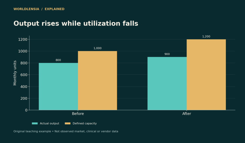
A fictional plant produces 800 units in a month against a defined sustainable capacity of 1,000. Its utilization is 80%. If capacity rises to 1,200 and output rises to 900, utilization becomes 75% even though production increased by 12.5%.
| Period | Actual output | Defined capacity | Utilization |
|---|---|---|---|
| Before expansion | 800 | 1,000 | 80% |
| After expansion | 900 | 1,200 | 75% |

Figure data and assumptions
Original hypothetical teaching data; see the caption and article for assumptions.
| Category | Actual output | Defined capacity |
|---|---|---|
| Before | 800.0 | 1000.0 |
| After | 900.0 | 1200.0 |
The lower rate does not prove a decline in demand or operational failure. The denominator expanded faster than output. The original chart separates output and capacity so this change remains visible.
Nameplate and sustainable capacity differ
A machine's theoretical maximum can assume uninterrupted operation under ideal conditions. A sustainable operating measure can allow for realistic schedules, normal downtime, and input availability. Neither should be substituted for the other without explanation.
If the capacity assumption changes, record the change. Adding shifts, changing product specifications, or revising expected downtime can alter the denominator. A series should not appear to improve merely because capacity was redefined downward.
The bottleneck controls the line
Suppose a production chain has three stages capable of 120, 80, and 100 units per hour. Without buffers or other complications, the 80-unit stage constrains steady output. Improving the first stage from 120 to 150 does not by itself raise the chain's limit above 80.
An average of stage capacities is not the line's capacity. Map the actual sequence and identify where work queues accumulate. A machine can be idle because an upstream stage starves it, not because its own demand is low.
Product mix can move the measure
One product may require twice as much time on the limiting machine as another. A unit count that treats them as identical can obscure the load. Use a measure appropriate to the resource being constrained, such as bottleneck hours, while keeping the assumptions clear.
If a plant shifts toward more complex products, output units can fall while resource utilization rises. This does not establish lower productivity or higher value without examining prices, labor, material, and quality outcomes.
High utilization has trade-offs
A tightly loaded process can have less room to absorb disruptions or urgent work. Maintenance, changeovers, supplier delays, and quality failures can affect achievable throughput. A target of 100% at every stage may not produce the best overall outcome.
Do not infer a universal safe utilization level from the fictional examples. The suitable operating range depends on variability, service requirements, process design, and the cost of spare capacity. Historical data from the actual operation are more useful than an unsupported benchmark.
Separate output from good output
Producing 1,000 units with a high defect rate is different from shipping 1,000 acceptable units. State whether the numerator counts gross production, finished goods, or saleable output. Rework can consume capacity while hiding the underlying quality issue.
Similarly, revenue is not a capacity measure. Higher prices can raise sales value without more physical throughput. Pair financial results with operational quantities when investigating whether additional equipment is needed.
Read national statistics at their own scale
An industrial utilization series summarizes multiple industries with its own estimation and aggregation methods. It can provide economic context but cannot identify a particular supplier's bottleneck. Sector averages may also conceal significant differences across plants.
For a business decision, combine the broader series with order books, delivery performance, maintenance logs, labor constraints, and the actual process map. Do not treat a national reading as a substitute for local due diligence.
Separate demand limitation from resource limitation
A plant can produce less than capacity because orders are weak, because inputs are unavailable, or because a critical stage fails. The same utilization ratio can arise from different causes. Check order backlog, materials, staffing, equipment availability, and scheduling before selecting a remedy.
If demand is the constraint, buying another machine may add unused capacity. If one scarce component is the constraint, a marketing campaign may increase unfulfilled orders. The ratio points to a gap; operational records explain why it exists.
Record temporary and structural conditions separately. A one-week outage can affect a monthly result without establishing that long-run capacity is lower. Conversely, recurring downtime may require revising an overly optimistic capacity assumption.

Figure data and assumptions
Original hypothetical teaching data; see the caption and article for assumptions.
| Category | Before | After stage 2 expansion |
|---|---|---|
| Stage 1 | 120.0 | 120.0 |
| Stage 2 | 80.0 | 110.0 |
| Stage 3 | 100.0 | 100.0 |
Test a proposed expansion against the bottleneck
Return to the fictional stages with hourly capacities of 120, 80, and 100. If the second stage is expanded to 110, the third stage's 100 becomes the new limit. The line improves from 80 to 100, not 110, under the simplified assumptions.
If management pays for 110 units of capacity at the second stage but expects 110 units of final output, the plan overlooks the next constraint. A process map makes this visible before committing resources.
This example assumes compatible product units, no yield loss, and no other restrictions. A real line may require buffers, changeovers, batch scheduling, and quality adjustments. The purpose is to demonstrate the sequence of constraints, not to provide a factory-design formula.
Staffing and equipment are not interchangeable
An available machine does not necessarily imply the trained staff needed to operate it. Adding shifts can require supervision, maintenance, support functions, and supply coordination. Include these in a realistic capacity estimate.
Likewise, increasing labor hours cannot always overcome a physical equipment limit. Distinguish theoretical machine output, staffed capacity, and actual throughput. A report that labels all three simply “capacity” makes it difficult to understand what an investment changes.
For service businesses, analogous constraints may involve specialist time, appointment slots, review queues, or software limits. Use domain-appropriate quantities rather than transferring a factory unit measure mechanically.
Utilization and efficiency need different labels
Utilization compares output with capacity. Efficiency can refer to output per input or performance relative to another defined standard. A facility can use much of its capacity while consuming more material or labor per saleable unit than expected.
Choose operational measures that identify the actual issue: throughput, yield, downtime, labor productivity, delivery time, and cost per acceptable unit. Reporting them together can explain why a busy plant is not profitable.
Avoid composite scores that combine these dimensions without revealing weights. A single improvement index may be convenient, but it can conceal worsening quality behind higher volume. Keep the component evidence available.
Connect the operating and financial cases
Suppose a proposed investment increases sustainable output by 200 units per month. At a contribution of $20 per unit, the maximum additional contribution under full incremental demand is $4,000 per month before new fixed costs. If the expansion adds $3,000 of monthly fixed costs, the simple operating gain is $1,000 under those assumptions.
That is not a full investment appraisal: upfront capital, financing, taxes, maintenance, risk, and demand uncertainty remain. It does show why additional capacity must be connected to contribution and realistic sales rather than celebrated as a physical number alone.
Use the break-even guide to test the required extra demand. Then check whether suppliers, labor, and downstream stages can actually deliver it. The strongest case reconciles the process map with the financial model.
Review the observation window
Hourly, monthly, and annual utilization can tell different stories. A process running near its limit for several hours may still have substantial unused time across the month. A monthly average can also hide peaks that cause late deliveries.
Keep the period consistent with the decision. A promise to fulfill a daily service window needs evidence about the relevant peak, not just an annual average. A long-term equipment investment may need a broader view of demand and sustainable operation.
Show a distribution or a peak measure when variability matters, and state how downtime is treated. Do not compare a peak rate with an average rate while using the same label.
Reconcile forecasts with completed periods
After an expansion, compare the promised capacity and output with actual results. Identify whether differences came from demand, implementation delay, product mix, quality, staffing, or another constraint. A useful review can improve the next estimate.
Keep the original forecast rather than replacing it with the latest assumption before assessing performance. That makes it possible to learn which parts of the operating model were realistic and which need better evidence.
A useful capacity report
Report output, capacity definition, time period, product mix, downtime treatment, quality, and the limiting resource. Explain whether a change came from output, the denominator, or both. Then compare proposed sales targets with feasible throughput.
WorldLensia's break-even analysis shows why this matters financially: a price discount can require a sales volume the operation cannot fulfill. A good plan tests profitability and physical feasibility together.
Avoid a universal utilization target
The fictional 80% rate is not a recommendation. A stable process, a highly variable service queue, and a seasonal factory can need different spare capacity. The cost of delays and the cost of unused resources also differ. A target should follow measured variability, service requirements, and realistic operating conditions. Explain those inputs before presenting a benchmark. If a published industry figure is used for context, identify its coverage and method, and do not assume it is a suitable operating target for an individual business with a different product mix or constraint.
Sources and methodology
Federal Reserve G.17 explanatory notes were checked October 18, 2026. The plant, capacities, and production-chain example are original hypothetical scenarios, not industrial survey observations.
- Federal Reserve: G.17 explanatory notes — checked October 18, 2026.
Continue with Inventory turnover and days on hand and Margin and markup for related context.
To connect capacity limits with replenishment and relevant costs, see Why Average Lead Time Is Not Enough for an Inventory Buffer and Allocated Cost and Incremental Cost Answer Different Decisions.