
Two suppliers can deliver in five days on average and still create very different inventory risks. One may arrive close to five days almost every time; another may alternate between unusually early and unusually late deliveries. The mean describes the center of those histories, not the exposure created by their variation.
An inventory buffer therefore needs a clearer question than “What is the average delay?” Define the demand period being protected, the replenishment process and the service objective. Then assess whether the available data can support the policy being considered.
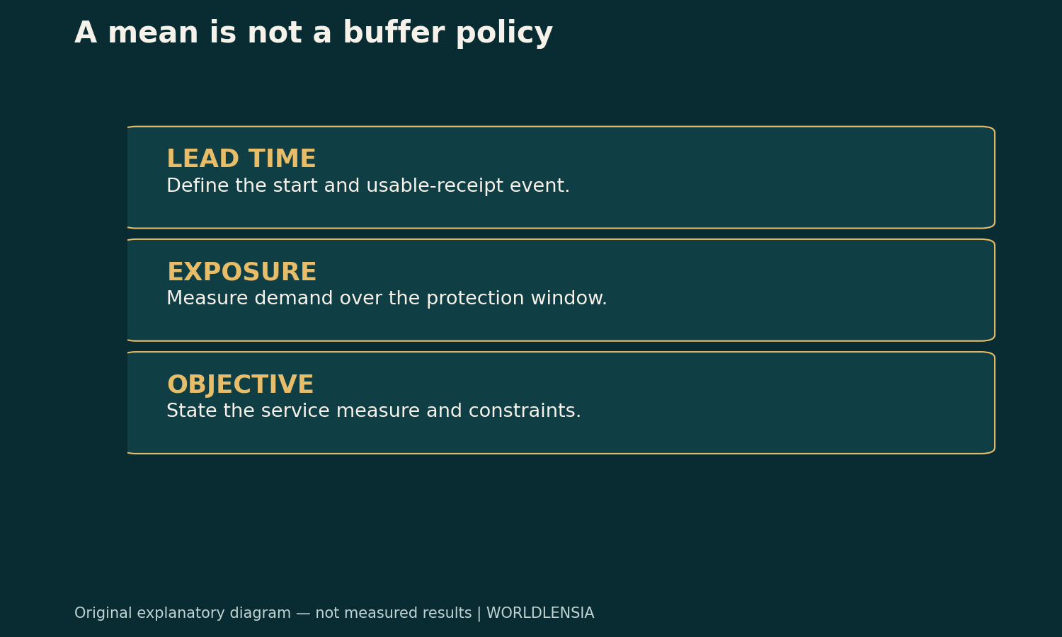
Define lead time from two named events
Lead time can begin when an order is approved, submitted, confirmed or dispatched, depending on the process. It can end at arrival, inspection or the moment stock becomes usable. Those are not interchangeable intervals.
If one supplier's record measures dispatch-to-arrival and another measures order-to-usable-stock, comparing their averages can mislead before variability is considered. Record the event definitions and include weekends, holidays or business-day conventions explicitly.
For an operating decision, use the interval during which the business must protect demand. An item physically delivered but waiting for required inspection may not yet be available to serve customers. The measurement should match the process rather than the easiest timestamp to export.
Equal means, different histories
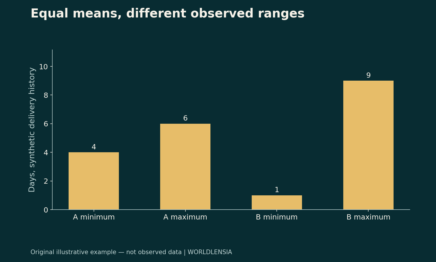
Consider two fictional suppliers with three observed delivery times each. Supplier A takes 4, 5 and 6 days. Supplier B takes 1, 5 and 9 days. Both averages are five days.
| Synthetic supplier | Delivery times | Mean | Observed range |
|---|---|---|---|
| A | 4, 5, 6 days | 5 days | 4–6 days |
| B | 1, 5, 9 days | 5 days | 1–9 days |
The records have the same center and different spreads. That observation does not prove how either supplier will behave next month. Three deliveries are too little evidence to characterize a reliable tail probability or a complete lead-time distribution.
The example establishes only why the mean is insufficient. It does not justify choosing a particular safety-stock quantity or declaring one supplier better overall.
Translate time into demand exposure
Assume, only for this teaching example, that demand is a constant ten units per day. Supplier A's observed lead times correspond to 40, 50 and 60 units of demand. Supplier B's correspond to 10, 50 and 90 units.
The expected exposure under the three-value arithmetic is 50 units for each. But an order point designed only around that average can face a larger observed late-delivery requirement in B's history.
Real demand is often variable, and demand during lead time is not necessarily independent of lead time. A busy season can affect both sales and supplier delays. Do not multiply two unrelated averages and assume the result captures the full uncertainty.
Keep the toy assumption visible. Its purpose is to connect days with units, not to propose a real inventory formula.
A buffer protects a stated objective
“Avoid stockouts” is not yet a complete measurable policy. A cycle-service objective concerns the chance of avoiding a stockout during a replenishment cycle under a defined model. A fill-rate objective concerns the share of demand fulfilled directly from stock under its definition.
Those objectives can produce different requirements. A policy can experience stockouts in several cycles yet still fill most units if the shortages are small. Conversely, a rare but large shortage can have a substantial unit impact.
MIT's stochastic-inventory teaching material provides the methodological foundation for connecting variability and service objectives. A business still needs an appropriate model and evidence for its particular demand, replenishment and cost conditions.
Do not infer a service probability from three points
In the fictional B history, one of three deliveries takes nine days. That does not establish that future nine-day delays occur with a stable probability of one third. The observations may not represent the season, supplier process or current operating conditions.
Use more relevant data and inspect how it was collected. Check missing deliveries, canceled orders, exceptional disruptions and whether late orders were excluded from the export. A clean average can be biased if the most difficult cases are absent.
Separate descriptive history from a fitted forecast. If an analyst assumes a distribution, record the assumption and test its consequences. Do not present model-based tail estimates as directly observed frequencies.
Replenishment timing adds another boundary
A continuously monitored inventory position and a system reviewed once a week can face different protection periods. In a periodic-review process, demand may occur before the next review as well as during the subsequent replenishment lead time.
Define when orders can be placed and how outstanding orders are counted. A policy that ignores stock already on order can over-order; one that ignores commitments to customers can overstate availability.
The relevant account is more than the physical units on a shelf. Document inventory position, pending receipts and known demand commitments using the system's definitions. Otherwise, a theoretically sensible buffer can be implemented against the wrong starting quantity.
Supplier choice includes more than variation
Delivery reliability is important, but it is not the only consideration. Price, minimum order quantity, quality, replacement terms, capacity and communication can affect the decision. The fictional mean-and-range table cannot settle that broader comparison.
Ask whether an apparently fast supplier delivers complete usable orders. A partial delivery can have a different effect from a complete one. Record the quantity and quality outcomes alongside timing if they affect service.
Avoid creating a composite supplier score with arbitrary weights and then presenting it as objective evidence. If a scoring system is used, identify whose priorities the weights express and test whether the decision changes under reasonable alternatives.
Buffers have costs and limits
Additional inventory can tie up cash, require storage and create obsolescence or spoilage exposure. Too little inventory can create lost sales, expediting work or service problems. The appropriate balance depends on the item and operating context.
Do not assume that a larger buffer solves every supply problem. Chronic quality failures, an unreliable ordering process or a capacity shortfall may need a different intervention. A buffer can absorb some variation without repairing its cause.
The inventory-turnover guide helps interpret how stock relates to activity. The cash-conversion-cycle guide explains why inventory decisions also affect when cash is tied up. Neither ratio alone supplies a safety-stock policy.
Build an evidence record for the policy
For each replenishment, retain the item, ordered quantity, order event, usable-receipt event, partial deliveries and relevant exceptions. Match demand observations to the same time basis. Keep a record of process changes so old data is not assumed to represent a new supplier arrangement.
State the service objective and how it is measured. Identify which costs are observed and which are assumptions. Test a proposed policy against a relevant historical or simulated sequence without using the same exercise as proof that future service is guaranteed.
Monitor the result after implementation. A change in demand mix or delivery behavior can make the previous buffer inappropriate. Review the data and objective rather than increasing stock automatically whenever one late delivery occurs.
A careful conclusion from the example
Both fictional suppliers average five days, but B's three observed deliveries span a wider range. Under constant ten-unit daily demand, that creates a wider observed exposure range. Those are the supported descriptive statements.
Selecting a buffer requires more: a relevant dataset, a defined replenishment process, a service objective and a model whose assumptions fit the decision. The average is a useful input, but it is not the entire inventory policy.
Do not confuse a longer mean with greater variability
A supplier can be consistently slower but less variable than another supplier. Mean and spread describe different features. A policy may respond to each differently, depending on the protection period, order cycle and service objective.
Keep both fields in the comparison. If a faster mean is accompanied by a wider tail, describe the tradeoff rather than declaring an unqualified improvement. If the available data cannot estimate the tail credibly, state that limitation.
The same applies to a before-and-after process change. Compare compatible periods and check whether a few extreme cases dominate the result. A summary should not erase the events that create the practical exposure.
Demand measurement needs a lost-sales boundary
Observed sales may not equal demand when stockouts prevent purchases. A history built only from completed sales can understate the demand the inventory policy was supposed to serve. Investigate how the system records unfilled requests or lost sales before treating the series as complete demand.
Do not invent missing demand. Use available evidence and an appropriate documented estimation method if one is needed. Mark estimated quantities separately from observed transactions.
This boundary can matter when evaluating a new buffer. Higher completed sales after an increase may reflect previously unmet demand, other business changes or a combination. A causal conclusion requires more than comparing two totals.
Test operational feasibility as well as the formula
A policy can be mathematically coherent and difficult to execute if order quantities, storage limits or supplier minimums prevent the proposed actions. Record those constraints before treating a model output as an instruction.
Check who reviews exceptions and how the inventory position is updated. Late or inaccurate receipts can undermine a policy even when its target quantity is reasonable. The operating process needs its own verification.
The practical objective is a decision rule that can be followed, monitored and revised with evidence. A single average lead time is one input to that rule, not a complete specification of it.
Keep units consistent
If demand uses business days and lead time uses calendar days, reconcile the time basis before multiplying them. A correct-looking product can otherwise describe the wrong exposure window. Label the chosen convention in the worksheet.
Sources and methodology
Inventory concepts were checked against MIT OpenCourseWare's Fall 2009 lecture on stochastic inventory models and supply contracts on October 19, 2026. All supplier histories, demand quantities and calculations are original hypothetical examples. No real supplier evaluation, calibrated stock recommendation or service guarantee is claimed.
To connect replenishment variation with turnover and bottlenecks, see Inventory Turnover and Days on Hand: Read the Ratio Carefully and Capacity Utilization: A Busy Factory Can Still Have a Bottleneck.